In the previous post, we explored the method of phase estimation where we recovered the phase factor \(\omega\) from the state
\[ \frac 1 {\sqrt{m}}\sum_{y = 0}^{m} \exp(2 \pi i \omega y)|y\rangle \] and we demonstrated that a quantum circuit consisting of Hadamard gates and controlled rotations can recover the binary digits of \(\omega\) in reverse order. If \(\omega\) is an integer multiple of \(1/2^n = 1/m\) where \(n\) is the number of qubits in the system, theoretically the phase estimation circuit yields the precise value of \(\omega\) after measurement. However, in practice, \(\omega\) is likely to be an arbitrary real value. In this post, we compute the probability of circuit collapsing to the correct answer where \(\omega\) is not necessarily an integer multiple of \(1/2^n = 1/m\).
Start with an analytical result which will come in handy later.
Lemma If \(M \theta \in [0, \pi/2]\), then \[\frac {1} {M^2} \frac{\sin(M\theta)^2}{\sin(\theta)^2} \geq \frac {4}{\pi^2}\]
Proof. By taking the derivative, it is easy to verify that the square root of the derivative is monotonically decreasing. The fact that \(\tan(x)\) grows more rapidly than \(x\) in the positive reals come in handy. Since the function is monotonically, the minimum is attained when \(\theta = \frac{\pi}{2M}\). Bound \(\sin(\theta)\) over \(\theta\) and evaluate at the edge of the interval. □
The phase estimation algorithm(\(QFT_m\)) is exactly the inverse of the phase estimation algorithm(\(PE_m\)). This trivially follows from the problem statement of the phase estimation algorithm. Alternatively, one can apply two transforms sequentially and simplify the double sum.
\begin{align} QFT_m |x\rangle & = \ \frac {1} {\sqrt{m}} \sum_{y = 0}^{m – 1} \exp(2\pi i xy / m)|y\rangle \\ PE_m |y\rangle & = QFT^{-1}_m |y\rangle \ = \ \frac {1} {\sqrt{m}} \sum_{x = 0}^{m – 1} \exp(-2\pi i yx / m)|x\rangle \end{align}
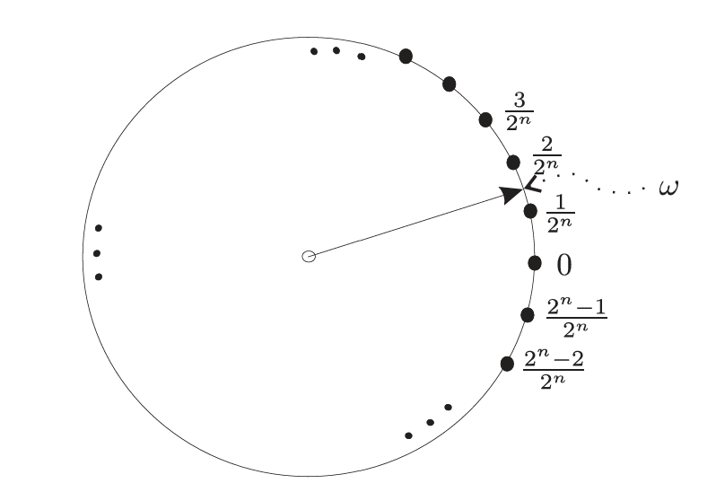
Suppose we are provided with a nonpure state that has a phase factor \(\omega\) which is not an integer multiple of \( 1/2^n\). Abuse notation and denote
\[ |\omega \rangle \ = \ \frac 1 {\sqrt{m}} \sum_{y = 0}^{m – 1} \exp(2\pi i \omega y) |y\rangle\]
Consider the \(QFT_m\) circuit as a basis transform. After running the circuit, the result is collapsed down to some integer multiple of \(1/2^n\). Let the multiplier \(x\) of the phase factor denote the orthonormal states, and denote them as \(|x\rangle\). The input state corresponding to the output state \(|x\rangle\) is
\[PE_m^{-1}|x\rangle \ = \ QFT_m|x\rangle \ = \ \frac 1 {\sqrt{m}} \sum_{y = 0}^{m – 1} \exp(2\pi i \omega y)|y\rangle\]
Assuming the Phase Estimation algorithm as a basis transform, we can use Born Rule to compute the probability that state \(|\omega \rangle\) will yield the phase \(x/m\) after QFT evaluation. The final state with respect to the new basis is \(QFT_m|x\rangle\) and the initial state is \(|\omega\rangle\). Thus,
\[P_{\omega\rightarrow x} \ = \ \| \langle \omega |QFT_m| x \rangle^2 \| \ = \ \| \frac 1 {m} \frac {1 – \exp(2\pi i \cdot (m \omega – x))}{1 – \exp(2\pi i (\omega – x / m))} \|^2 \ = \ \frac 1{m^2} \frac{\sin(\pi (m \omega – x))^2} {\sin(\pi (\omega – x / m))^2} \]
If the phase \(\omega\) is evaluated to the nearest integer multiple of \(1/m\), then the argument \(m\pi (\omega – x/m)\) is guaranteed to be less than \(\pi/2\). Applying the analytical result from above, we conclude that the probability that Phase Estimation yields the closest approximation is \(4 / \pi \approx .405\) Also, the quantity \(m \omega \) can be approximated from both under and over that satisfies the phase bounds. Losely, the phase approximation is accurate with a probability of \(8 / \pi \approx .811\).
Leave a Reply